
Abstract: This article reviews two significant structural changes in the inflation formation mechanism in China since 1980 and probes into the reasons behind them. The first was around 1996, when the price of manufactured goods in China began to move in tandem with that in the United States as a result of China’s opening up and a stable Chinese yuan. The second was around 2013, when food price’s influence on total consumer prices and manufactured goods prices plummeted or even disappeared, while the non-food price had a closer correlation with economic growth. The reason was that China passed the second Lewis turning point when wage pressure on non-food producers with slower productivity growth was increasingly manifested as price hikes, thus establishing a stable correlation among economic growth, wage growth and non-food inflation.
The inflation formation mechanism in China, while highly consistent with economic theories, shows many unique features.
The Chinese economy has undergone tremendous transformations over the past four decades, achieving extremely rapid growth and approaching the level of high-income economies this year. During the process, China has made great headway in opening up and transforming from a planned economy to a market economy, from agriculture-dominated to industry- and service-led, and from one with the rural population as the majority to a highly urbanized country.
The transformations have been accompanied by critical structural changes in the country’s inflation formation mechanism. An in-depth analysis of these evolvements could shed light on the tremendous growth and changes China has experienced over the past 40 years and help us understand the formation of inflation today.
I. THE OPENING-UP OF THE CHINESE ECONOMY
One particular structural change has played an essential part shaping the inflation formation mechanism in China.
Look at the producer price for manufactured goods in China and the United States during 1980-1996. Before 1983, China still implemented rigid price control under the planned economy system; but after the mid-1980s, the control was gradually lifted with more volatile market-driven price fluctuations.
The price also experienced several drastic changes during this period. However, over the 16 years, this price in the two countries had no close relationship, with a correlation coefficient of -0.2.
Nevertheless, after 1996, the producer price for manufactured goods in China and the U.S. began to show robust correlations, with the coefficient surging to 0.92. Over the 26 years, all rises and falls in the price have been completely synchronized in the two countries. The price in China and the U.S. peaked and bottomed at about the same place.
As shown in Figure 1, the year of 1996 marked a watershed.
What has given rise to such synchronism?
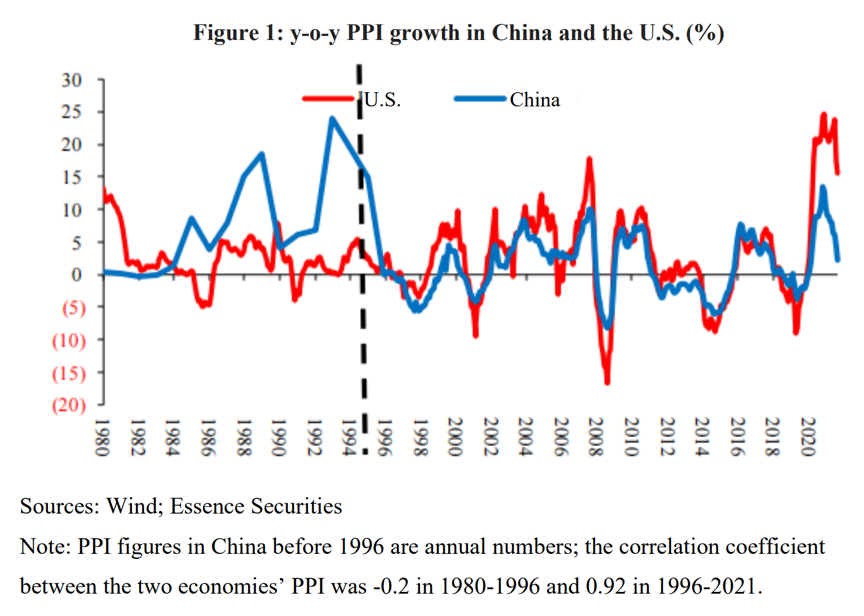
The reason was simple: 1) China accelerated its opening-up in the 1980s and has integrated into the world economy rapidly since the 1990s; 2) China liberated foreign exchange transactions under the current account in 1996 and has kept the Chinese yuan (CNY) stable against the greenback.
Under such conditions, the law of one price (LOOP) came into play. If the iron price in China is significantly higher than the global price, Chinese importers could bring in much iron manufactured abroad which would then pare down the domestic price to the global level. Thus, the PPI in China and the U.S. began to move in tandem with each other.
The phenomenon indicates that as China rapidly integrated into the world economy and when the CNY remained relatively stable, the price fluctuations of tradable goods and manufactured goods in China soon became part of the global manufactured goods price changes.
Against this backdrop, if we were to understand the changes in the producer price for manufactured goods in China, we must look at global economic and geopolitical evolvements, as well as changes in the monetary policies of major economies around the world.
II. FOOD INFLATION-DRIVEN CPI
Next, look at the relationship between food inflation and the general consumer price.
Figure 2 shows three data series, or mainly two. The red line indicates fluctuations in China’s consumer price index (CPI); the blue line represents CPI excluding food prices.
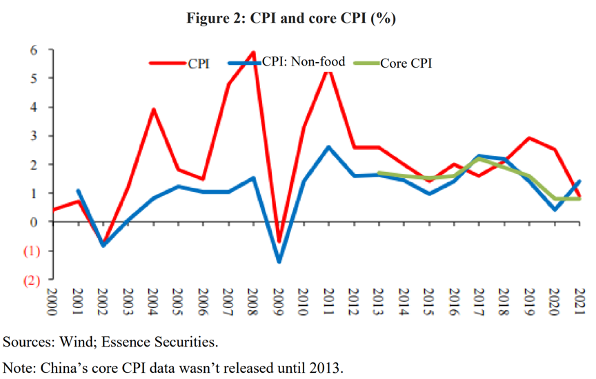
In this period, the first important fact is that average annual growth of non-food inflation in China remained low and steady, mostly within the range of 0-1.5%. But at the same time, the total CPI was highly volatile.
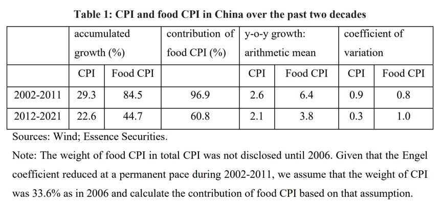
As the table shows, during 2002-2011, China recorded an average annual CPI growth of 2.6%, whereas food CPI increased at an annual average 6.4%, 97% of total growth. CPI excluding food increased annually at only 0.7% with minor fluctuations.
The second important fact is that during 1996-2012, the prices of food and manufactured goods moved highly consistently with a correlation coefficient of 0.77.
As said above, the price of manufactured goods in China is part of the global price, so the consistency is entirely unexpected.
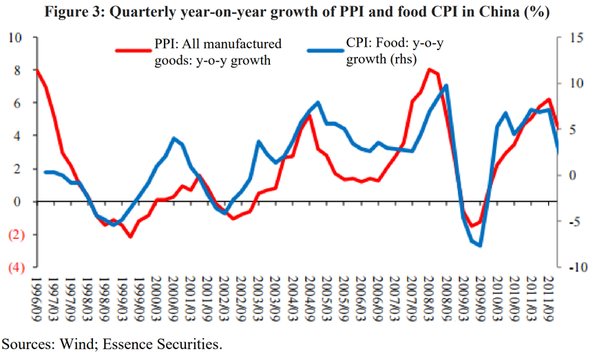
One explanation is that food price is determined by supply, core factors being weather conditions, crop harvest, and livestock diseases. If this is true, then food price fluctuations would be “noises” for the macro economy, but its strong synchronism with the price of manufactured goods hardly supports this view.
The second explanation is cost transmission: manufactured goods are essential raw materials for food production, including fertilizers, seeds, pesticides, agricultural equipment, and transportation. The rise in the price of manufactured goods has pushed up the cost of food production.
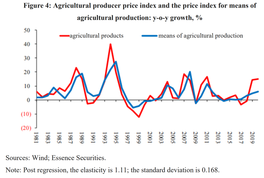
Let us first observe the PPI for agricultural products and the price index for means of agricultural production. Their consistency is not unexpected; what is unexpected, though, is that they have an elasticity of 1.1, meaning that with a 10% rise in the price for means of agricultural production, the price for agricultural products will increase by 11%, which does not support the cost transmission assumption, since means for production is not the only input. There are other inputs including land and labor.
Assuming that means of agricultural production account for 70% or lower in total agricultural production cost, considering cost transmission only, their elasticity should be at most 0.7. So, we can rule out the cost transmission assumption, too.
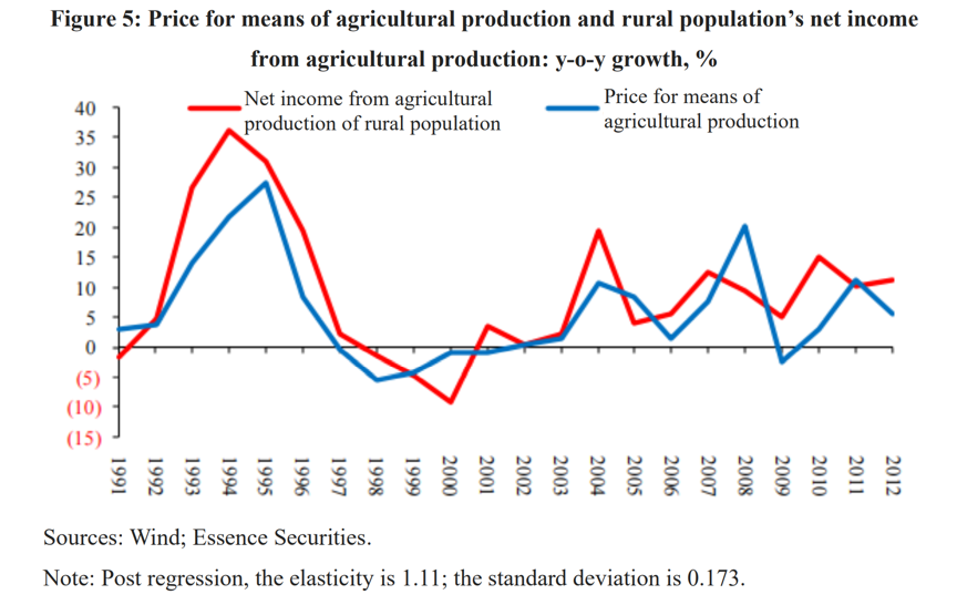
There is another piece of evidence. The elasticity between the rural population’s net per-capita income from agricultural production and the price for the means of agricultural production is 1.14, also higher than 1. Each time when means for agricultural production gets more expensive, the income of rural households from agricultural production rises at an even faster pace. This counters the cost transmission assumption, too.
The third explanation is that fluctuations in the price of agricultural products results from inflation expectations. When farmers see a higher price for agricultural production, they form inflation expectations and believe that agricultural products will become expensive as well. That leads them to increase inventory and reduce sales, causing a supply strain immediately.
Considering the relatively stable demand for agricultural products, this pushes up prices almost at once. This is inflation expectation transmission.
This was first proposed by Professor Song Guoqing at Peking University when he studied the 1994 inflation in China back in the 1990s. It is very insightful but has not been widely recognized for a long time.
Is there any exclusive evidence in support of the assumption of inflation expectation?
If inflation expectation and inventory adjustment are important mechanisms, then the price for hard-to-store agricultural products should be irrelevant to the price of manufactured goods; that for easy-to-store ones should be highly relevant.
In Figure 6 below, to the left are agricultural products with a higher correlation coefficient that is storable for more flexible inventory adjustment, while to the right are hard-to-store ones.
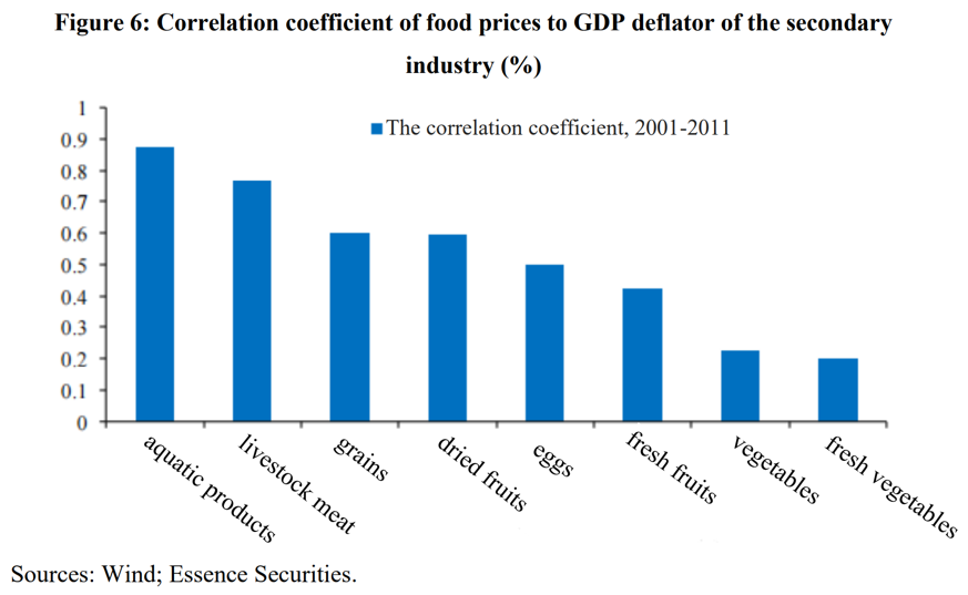
The most storable are grains, followed by dried fruits, eggs, fresh fruits, vegetables, and fresh vegetables. For livestock meat, except for refrigerated storage, another method is to delay the slaughter and marketing of pigs.
We could further examine the elasticity between these products’ prices and manufactured goods.
As shown in Figure 7, similar to the correlation coefficient, those whose inventory is easily adjustable have higher elasticity. This cannot be explained by crop harvest due to varying weather conditions or the cost of production.
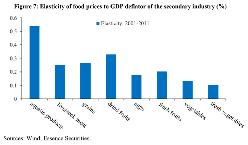
The above analysis is more favorable to the inflation expectation assumption.
III. NON-FOOD INFLATION HAS BECOME INDICATIVE
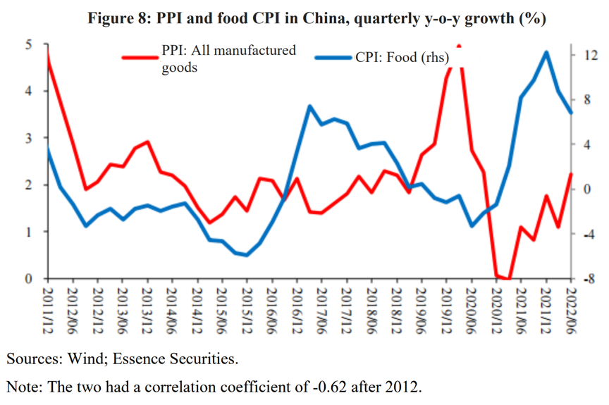
As mentioned above, during 1996-2012, food price and manufactured goods price moved highly in tandem, which, however, was no longer the case since 2012, as depicted in Figure 8.
Over the past decade, the two had a correlation coefficient of -0.62, sharing a solid negative correlation after 2016.
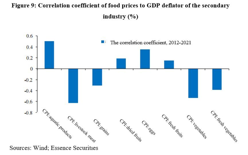
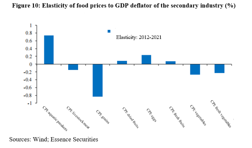
Moreover, as shown in Figures 9 and 10 below, the previous pattern in the elasticity and correlation between food price and manufactured goods price fluctuations has also disappeared over the past decade.
These developments indicate that inflation expectation and agricultural goods inventory adjustment mechanisms no longer played a significant role after 2012.
At the same time, as shown in Table 1, during 2012-2021, CPI rose by an accumulated 22.6%, 60% of which was from food, the dominating contributing factor, but significantly down from 97% a decade ago.
CPI in China was also much steadier. A decade ago, its coefficient of variation was 0.9, much higher than 0.3 now, mostly as a result of the lower contribution from food.
Meanwhile, core inflation rose remarkably. Non-food inflation included energy, but it was regarded as the closest measure to core inflation. A decade ago, China’s core inflation averaged 0.7%, much lower than 1.5% today.
Given that the decade from 2012 to 2021 saw slower economic growth with a rise in the price of most goods far lower than before, the rise in core inflation is even more notable and thought-provoking.
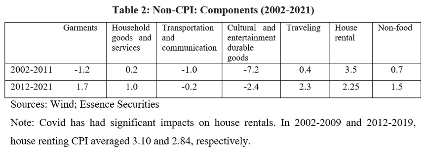
If we look at the components of core inflation, as shown in Table 2, many of them have experienced price hikes, so it is not because of abnormal fluctuations in some of the components.
As a matter of fact, in these components, only house rentals had slower growth, while all the others were increasing faster.
At the macro level, if we view food, industrial goods, and labor as inputs into non-food production, then is the increased price hike of non-foods a result of higher costs?
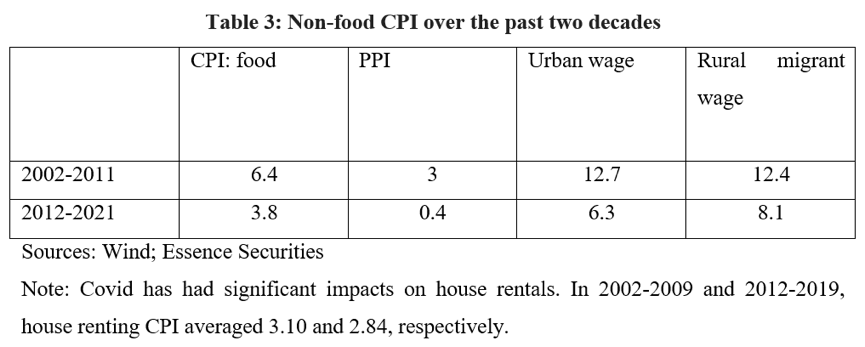
As shown in Table 3 below, the price of all these inputs had lower price hikes in the following decade, making the acceleration of non-food inflation even more abnormal.
The key reason behind is that the Chinese economy passed the second Lewis turning point in around 2013 (see Figure 11).
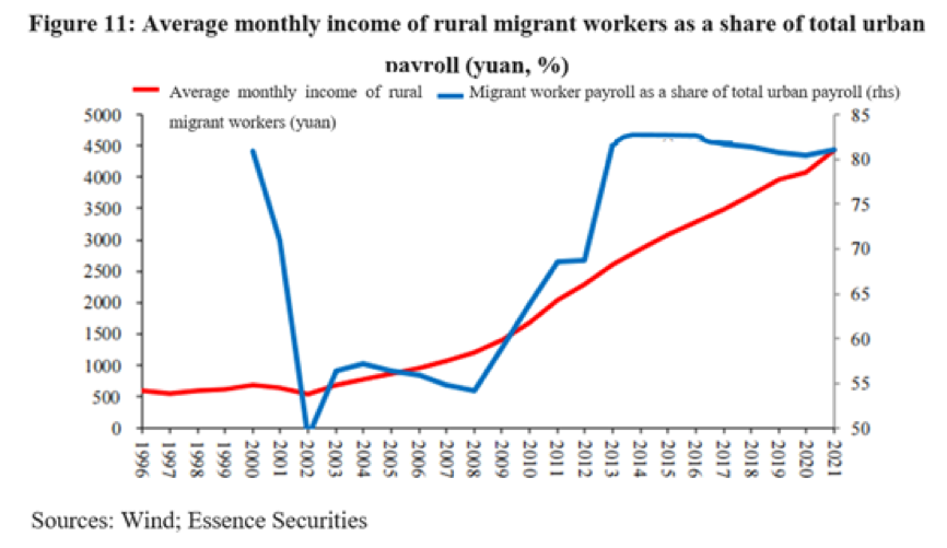
China passed the first Lewis turning point around 2005. Before 2005, low-end labor payroll adjusted for inflation remained stable; but after 2005, it began to surge.
However, before arriving at the second Lewis turning point, low-end laborers’ payroll was still lower than their marginal output in the industrial and service sectors. So, these sectors had greater motivation to employ more low-end laborers. This has led to a rapid increase in employment and/or an accelerating wage rise while putting continuous downward pressure on product market prices.
In the tradable goods market, the global price level is determined by the supply-demand balance. For price-taker economies, such pressure is manifested as rising competitiveness, increasing market share, and currency appreciation.
In the non-tradable goods market, such pressure is manifested as price signals.
This is not to say that the economy will not bear inflation pressure before it arrives at the second Lewis turning point; instead, it is to say that the inflation pressure during such period mainly comes from production capacity bottlenecks as a result of capital shortage.
After the economy passes the second Lewis turning point, the labor market would reach equilibrium, with wage equaling marginal output and the systemic downward pressure on non-tradable goods prices disappearing.
In the long run, if the productivity of tradable goods providers grows faster than that of non-tradable goods providers and the increase in labor payroll stands somewhere in between under equilibrium (equaling the growth of tradable goods considering exchange rate factors), then non-tradable goods providers will see faster price hikes.
Figure 12 below exhibits the productivity growth of various industries in China.
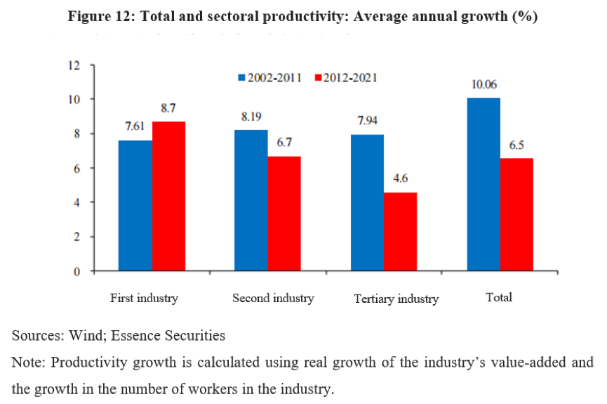
As shown in Table 3, during 2002-2011, wage growth averaged around 12.5%, much higher than the average annual growth of total productivity or that of the second and tertiary industries. But over the decade, the competitiveness of tradable goods providers boosted, whereas the non-tradable sector saw shallow price growth, if not deflation.
In the decade, the growth of labor payroll reduced to 6.3% (urban) and 8.1% (rural migrant workers); productivity of the second industry increased at 6.7%, much faster than the tertiary industry (4.6%). Export competitiveness improves slower, while non-tradable goods providers began to feel more price pressure.
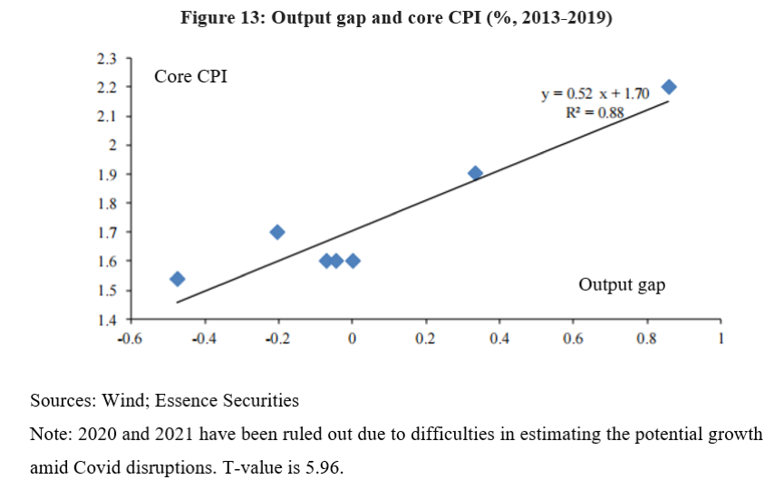
After the economy passed the second Lewis turning point, the labor market reached equilibrium, with a stronger correlation between core inflation and the output gap. The reason is that when economic growth accelerates, wage increases pick up at a faster pace than the productivity growth of non-tradable goods providers, thus adding to upward price pressure, which is then manifested as the price hike of non-food goods. The latter is much less reliant on tradable goods price than non-tradable goods price.
Figure 13 below shows the correlation between the output gap and the core inflation during 2013-2019 according to our calculation. The output gap is calculated as the average in the two years before and after a given timing (see Appendix). The period after 2020 is excluded to rule out the impact from Covid.
IV. CONVERGENCE OF URBAN AND RURAL RESIDENTS' LIFESTYLES
After the economy passes the second Lewis turning point, the price of low-wage labor rises to its marginal output so that the labor markets in urban and rural regions become integrated, implying significant economic development. At this point, rural households’ production and business behavior becomes part of the market adjustment process broadly. Rural households are no longer self-sufficient and isolated individuals, and their asset allocation starts to converge with that of urban residents.
Let’s see if there is some micro-evidence to support these judgments.
1. Changes in household food expenditure and international comparison
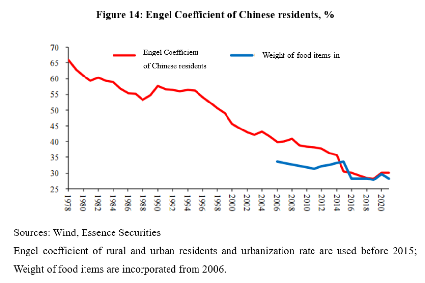
Since 1978, the share of food in residents' expenditures has fallen from 65% to less than 30% in China thanks to the country’s rapid economic growth and a substantial rise in per capita income. The significant decline in the Engel coefficient (see Figure 14) reflects the rapid improvement in living standards.
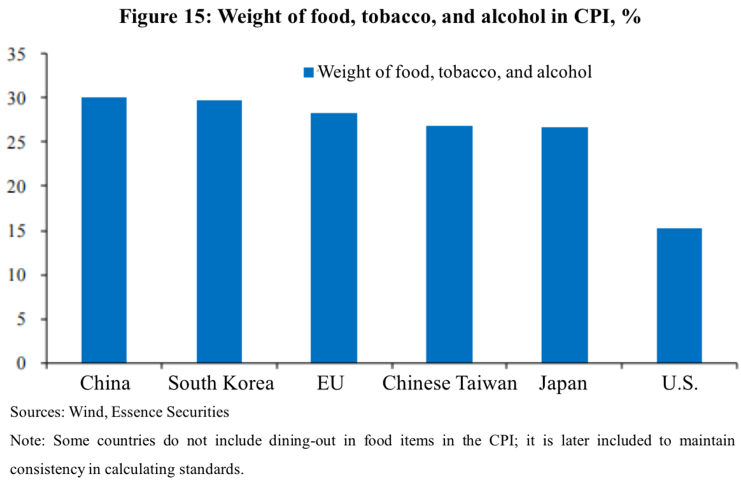
International comparisons also support the above statement. As shown in Figure 15 below, the share of food, tobacco, and alcohol in consumer spending of Chinese residents is already close to that of highly developed economies such as the European Union, Japan, South Korea, and Chinese Taiwan.
According to World Bank standards, China's per capita income last year was roughly only 4% short of the World Bank-defined threshold for high-income countries. If we look at the share of food expenditure, China is very close to the developed economies.
2. Changes in the spending behavior of rural households
Now let us look at the proportion of cash used in the spending of rural residents. Non-cash expenditures generally correspond to self-production and self-use, such as living in their own houses and eating food and vegetables. In general, the larger the proportion of non-cash expenditures, the closer the lifestyle is to self-sufficiency. A higher share of cash use indicates a more extensive and profound participation in the production and exchange process of the market.
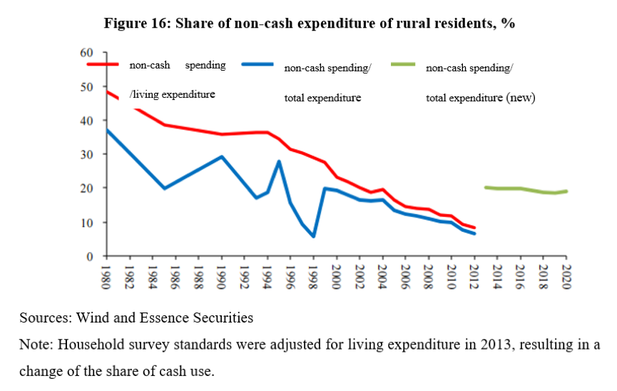
As shown in Figure 16 above, rural residents did not need cash for about half of their living expenses in 1980, while the ratio fell to 10% in 2012 (non-cash share of subsistence consumption) and 20% with the new standard. The rural households need to purchase 80% of consumer goods, so they are already part of the market division and transaction system.
As for urban residents (see Figure 17), they also have non-cash expenditures, mainly because they do not have to pay for their own homes. In addition, with the improvement of social security and medical insurance, the ratio of non-cash spending on medical consumption has increased, superimposed on the increase in medical consumption, jointly contributing to the increase in non-cash spending of urban residents. Rural residents undergo a similar situation.
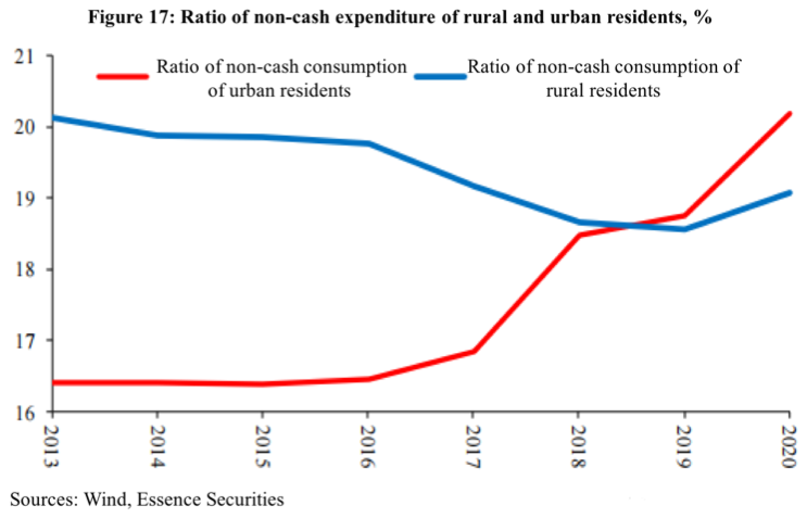
As can be seen, the share of cash use in consumer spending of rural and urban residents is generally similar after 2018, indicating a convergence of consumption patterns between urban and rural residents.
3. Changes in asset allocation of rural households
Now let us look at the changes in rural residents' savings allocation. Savings here are defined as income that is not consumed and can be allocated for bank deposits, agricultural inventories, homes building, farmland improvements, and agricultural equipment.
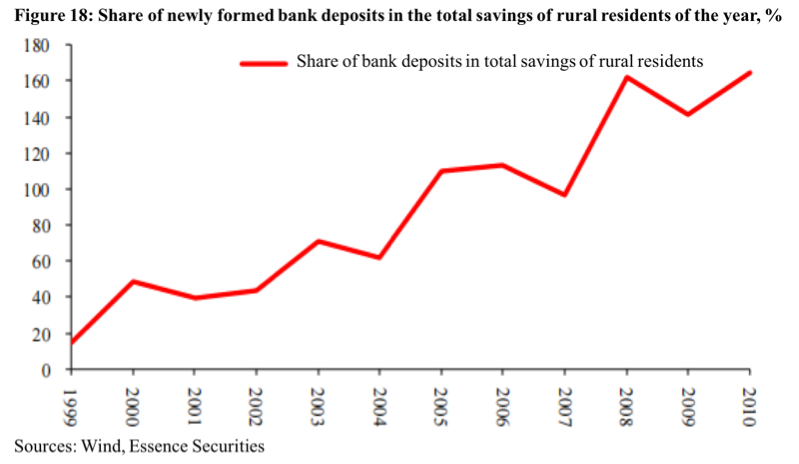
We examine the share of bank deposits to the total savings of rural residents as a measure of the extent to which their income balances become part of the financing process of the banking system.
As shown in Figure 18 below, this share was below 50% until 2002, approaching 100% in 2007 and reaching 150% after 2009.
Obviously, in the early years, a significant portion of savings was used for fixed asset formation and related productive activities in rural agriculture. In contrast, in the later years, all of the savings became part of bank financing.
Why did this ratio rapidly grow beyond 100% after 2008?
There is only one explanation, that in general the farmers disposed and sold their assets and had them deposited in the bank accounts.
One possibility is demolition. The government acquired houses and land of farmers in the suburbs, a process equivalent to asset disposal by farmers, and the income obtained from the process manifested itself in the form of bank deposits.
A second possibility is that, with the explosive growth of migrant wages before the second Lewis turning point, engaging in activities such as farming in the countryside is no longer plausible economically. Hence, farmers stop making new inputs or even dispose of their assets and leave the country for the cities.
Let us look at a critical case, pig farming.
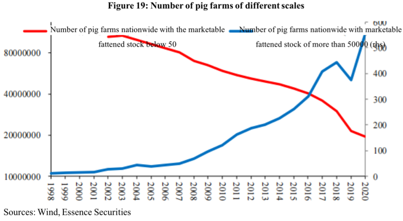
We assume farms with marketable fattened stock below 50 as small-scale free-range farming, and greater than 50,000 as industrial pig farming.
As shown in Figure 19, the number of small-scale free-range farms has continuously declined while that of intensive pig farming increased over the past 20 years. The sharp decline in free-range farming occurred around 2015.
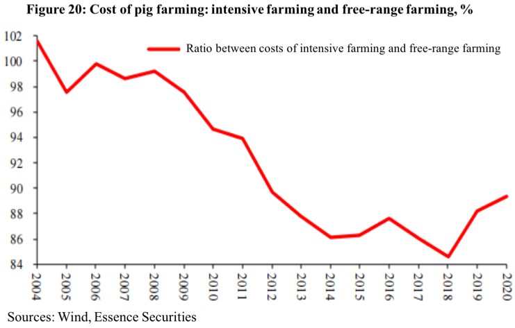
As shown in Figure 20, the costs of intensive and free-range pig farming were the same until 2008. The cost of intensive farming began to decline intensively and stabilized at about 85% of free-range farming after 2014. With this significant cost difference, free-range farmers started to sell their stocks and farms and deposited the money received in their bank accounts.
This evidence generally suggests that after the economy passed the second Lewis second turning point, the economic behaviors of urban and rural residents gradually converged. Rural households no longer held inventory as the main way to allocate their assets, thus explaining the disconnection between industrial products and food prices after 2012.
APPENDIX:
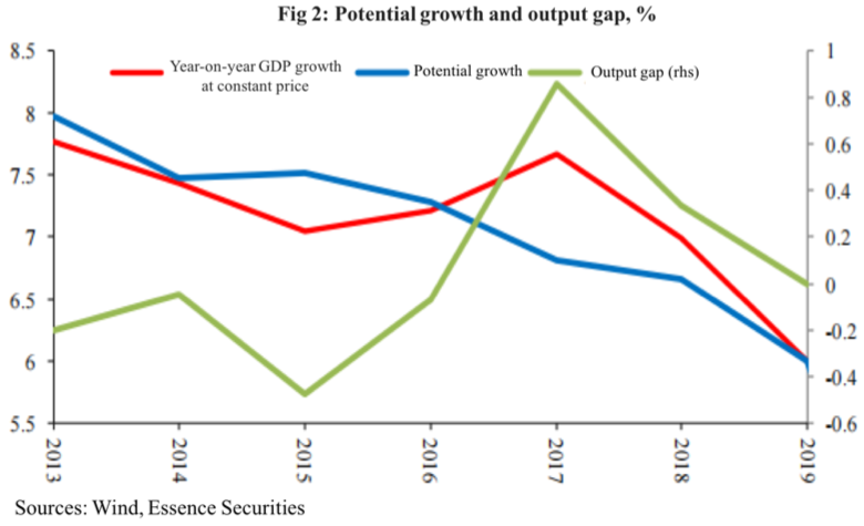
For calculating the output gap, we apply the moving average to calculate the potential growth rate for the current year. The average of the GDP growth rates of the two previous and two subsequent years (a total of 4 years) is taken as the potential growth rate for the current year. When estimating the potential growth rates of 2018 and 2019, anomalies in 2020 and 2021 are taken into account. It is assumed that the GDP growth rates of 2020 and 2021 would be 5.75% and 5.5% in the absence of the pandemic.
In addition, the supply-side reform has significantly dampened some sectors, leading to an abnormal decrease in industrial value added in 2016-2018. So the GDP data for 2016-2018 are adjusted accordingly.
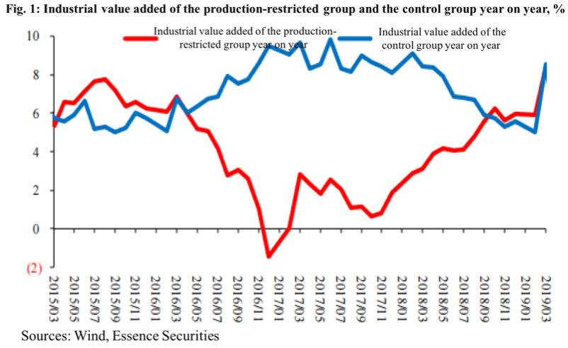
The GDP growth rates for 2016-2018 before and after the adjustment are shown in the table below.

The adjusted output gap and potential growth rate are shown below.
This is the speech made by the author at Peking University HSBC Business School in October 2022. It is translated by CF40 and has not been subject to the review of the author himself. The views expressed herewith are the author’s own and do not represent those of CF40 or other organizations.